Next: A.3 Iterative mean
Up: A. Statistical tools
Previous: A.1 Bayes' theorem
A.2 Maximum likelihood
The maximum likelihood principle is illustrated in an example with a one-dimensional data distribution {xi},
i = 1,..., n. We assume that the data originate from a Gaussian distribution p(x) with parameters  and
and  ,
,
According to the maximum likelihood principle,
we will choose the unknown parameters such that the given data are most likely under the obtained distribution. The probability L of the given data set is
L( , , ) = ) =  p(xi) = p(xi) =    exp exp - - 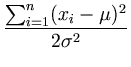  . . |
(A.4) |
We want to find
 and
and  that maximize L. Maximizing L is equivalent to maximizing log L, which is also called the log-likelihood
 ,
,
 (,) = log L(,) = - n log - (,) = log L(,) = - n log -  + const . + const . |
(A.5) |
To find the maximum we compute the derivatives of the log-likelihood
and set them to zero:
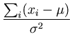
 |
= |
-  + +   0 , 0 , |
(A.6) |
 |
= |
 0 . 0 . |
(A.7) |
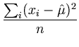
Thus, we obtain the values of the parameters
and :
The resulting
 is the variance of the distribution and is its center. The extremum of
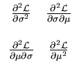
is indeed a local maximum, as can be seen by computing the Hesse matrix of
and evaluating it at the extreme point
(,):
is the variance of the distribution and is its center. The extremum of
is indeed a local maximum, as can be seen by computing the Hesse matrix of
and evaluating it at the extreme point
(,):
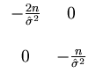
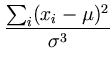
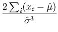
  |
= |
 - -  = - = -  = - = -  , , |
(A.11) |
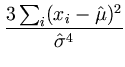
| |
|
|
|
 |
= |
 = - = -  = 0 , = 0 , |
|
| |
|
|
|
 |
= |
- . |
|
It follows that the Hesse matrix at the extremum is negative definite,
Therefore, the extremum is a local maximum. Moreover, it is also a global maximum. First, for finite parameters, no other extrema exist because
is a smooth function. Second,
is positive for finite parameters, but approaches zero for infinite values. Thus, any maximum must be in the finite range.
Next: A.3 Iterative mean
Up: A. Statistical tools
Previous: A.1 Bayes' theorem
Heiko Hoffmann
2005-03-22

 ,
, .
.